1
Machine Learning for Design
Lecture 7
Design and Develop Machine Learning Models - Part 1
2
Previously on ML4D
3
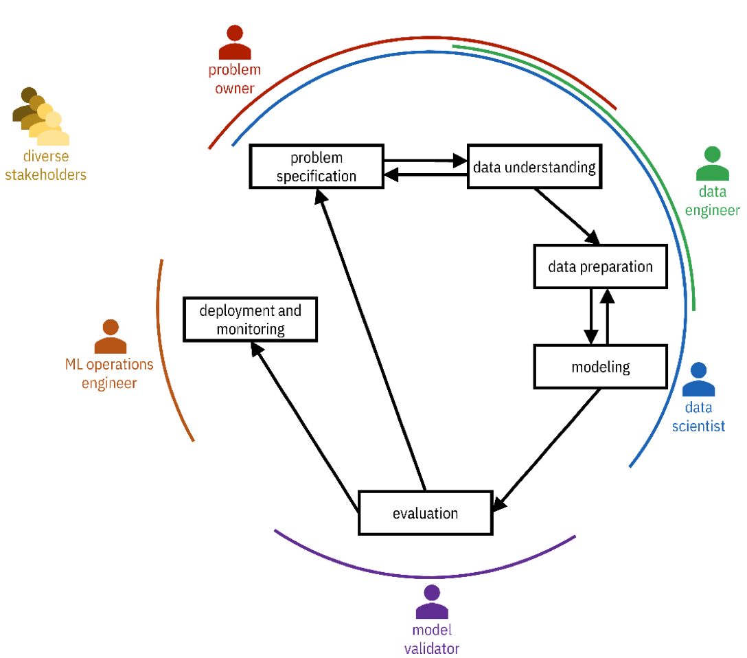
CRISP-DM Methodology
4
Data

5
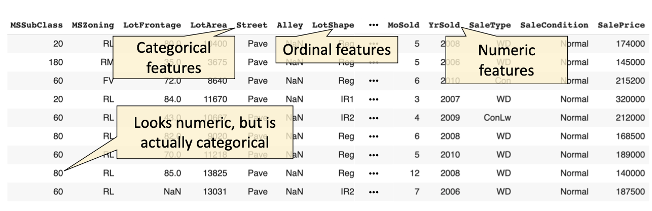
Types of Features / Label Values
- Categorical
- Named Data
- Can take numerical values, but no mathematical meaning
- Numerical
- -Measurements
- Take numerical values (discrete or continuous)
6
Categorical Nominal
- No order
- No direction
- e.g. marital status, gender, ethnicity
Categorical Ordinal
- Order
- Direction
- e.g., letter grades (A,B,C,D), ratings (dislike, neutral, like)
7
Numerical Interval
- Difference between measurements
- No true zero or fixed beginning
- e.g., temperature (C or F), IQ, time, dates
Numerical Ratio
- Difference between measurements
- True zero exists
- e.g., temperature (K), age, height
8
Data Preparation
9
Ideal Data
10
Real Data
11
- Data is rarely “clean”
- Approximately 50-80% of the time is spent on data wrangling
- probably an under-estimation
- Having good data with the correct features is critical
12
- 3 issues to deal with:
- Encoding features as numerical values
- Transforming features to make ML algorithms work better
- Dealing with missing feature values
13
Data Encoding
14
Numerical Features
Each feature is assigned its own value in the feature space
15
Categorical Features
- Why not encode each value as an integer?
- A naive integer encoding would create an ordering of the feature values that does not exist in the original data
- You can try direct integer encoding if a feature does have a natural ordering (ORDINAL e.g. ECTS grades A–F)
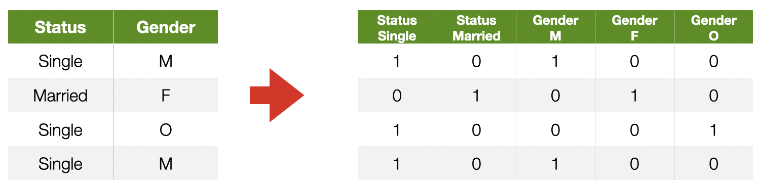
16
One-hot Encoding
Each value of a categorical feature gets its own column
17
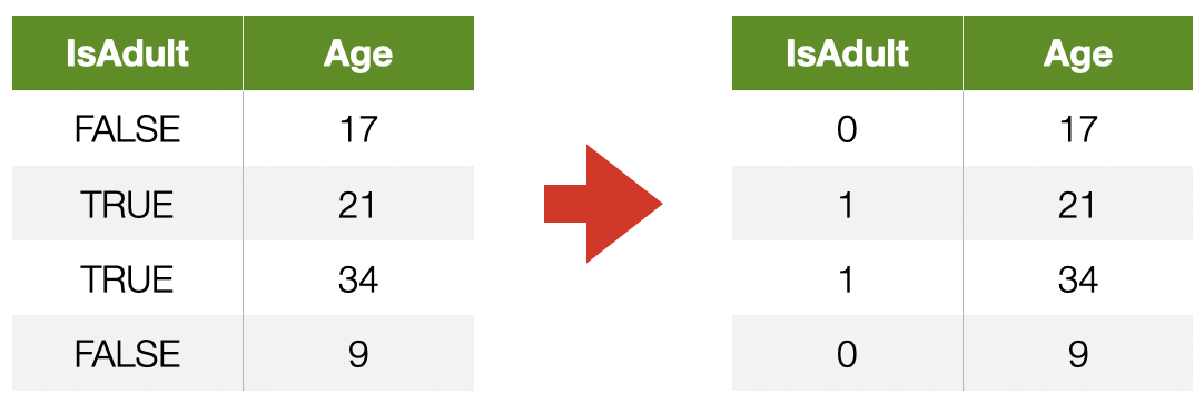
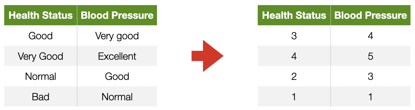
Ordinal Features
- Convert to a number, preserving the order
- —>
Encoding may not capture relative differences
18
Data Quality Issues
19
Incorrect feature values
- Typos
- e.g., color =
- Garbage
- e.g., color = “wr╍śïį”
- Inconsistent spelling (e.g., “color”, “colour”) or capitalization
- Inconsistent abbreviations (e.g., “Oak St.”, “Oak Street”)
20
Missing labels (classes)
- Delete instances if only a few are missing labels
- Use semi-supervised learning techniques
- Predict the missing labels via self-supervision
21
Merging Data
- Data may be split across different files (or systems!)
join based on a key to combine data into one table

22
Problems During Merge
- Inconsistent data
- Same instance key with conflicting labels
- Data duplication
- Data size
- Data might be too big to integrate
- Encoding issues
- Inconsistent data formats or terminology
- Key aspects mentioned in cell comments or auxiliary files
23
Dealing With Missing Values
24
Why can data be missing?
- "Good" reason: not all instances are meant to have a value
- Otherwise
- Technical issues (e.g. Data Quality)
25
Dealing with missing data
- Delete features with mostly missing values (columns)
- Delete instances with missing features (rows)
- Only if rare
- Feature imputation
- “fill in the blanks"
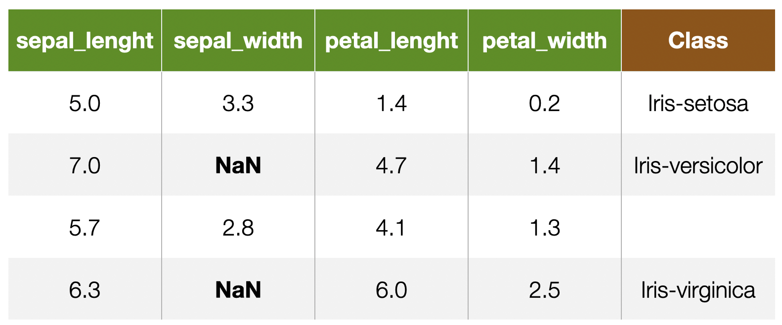
26
Feature Imputation
- Replacing with a constant
- the mean feature value (numerical)
- the mode (categorical or ordinal)
- “flag” missing values using out-of-range values
- Replacing with a random value
- Predicting the feature value from other features
27
What if our features look like this?
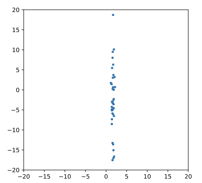
28
- What if the features have different magnitudes?
- Does it matter if a feature is represented as meters or millimetres?
- What if there are outliers?
- Values spread strongly affect many models:
- linear models (linear SVC, logistic regression, . . . )
- neural networks
- models based on distance or similarity (e.g. kNN )
- It does not matter for most tree-based predictors
29
Feature Normalisation
- Needed for many algorithms to work properly
- Or to speed up training
30
Min/Max Scaling
- Values scaled between 0 and 1
- and need to be known in advance
31
Standard Scaling
- Rescales features to have zero mean and unit variance
- Outliers can cause problems
32
Scaling to unit length
- Typical for textual document
33
Other features transformation
- Improve performance by applying other numerical transformation
- logarithm, square root, . . .
- TF-IDF
- It depends a lot on the data!
- Trial and error
- Exploration
- Intuition
34
Feature Selection and Removal
- Problem: the number of features may be very large
- Important information is drowned out
- Longer model training time
- More complexity --> bad for generalization
- Solution: leave out some features
- But which ones?
- Feature selection methods can find a useful subset
35
Feature Selection
- Idea: find a subspace that retains most of the information about the original data
- Pretty much as we were doing with word embeddings
- PRO: fewer dimensions make for datasets that are easier to explore and visualise, and faster training of ML algorithms
- CONS: drop in prediction accuracy (less information)
- There are many different methods, Principal Component Analysis is a classic
36
Principal Component Analysis
- Idea: features can be highly correlated with each other
- redundant information
- Principal components: new features constructed as linear combinations or mixtures of the initial features
- The new features (i.e., principal components) are uncorrelated
- Most of the information within the initial features is compressed into the first components

37
Principal Component Analysis
- Orthogonal projection of data onto lower-dimension linear space that:
- Maximizes the variance of projected data (purple line)
- Minimizes mean squared distance between data point and projections (sum of red lines)
38
Dimensionality Reduction
- Use the PCA transformation of the data instead of the original features
- Ignore the components of less significance (e.g., only pick the first three components)
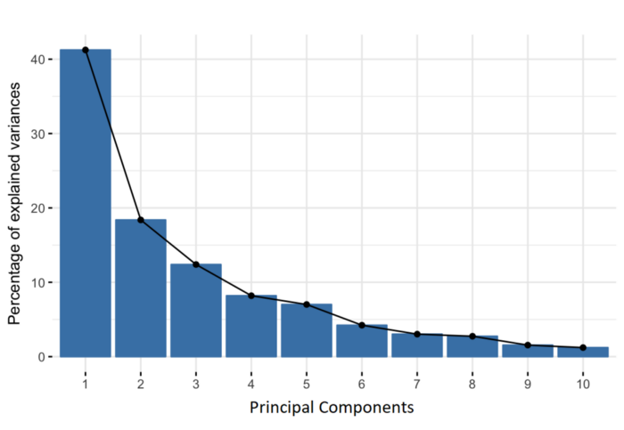
- PCA keeps most of the variance of the data
- So, we are reducing the dataset to features that retain meaningful variations of the dataset
39
And now, let's Smell Pittsburgh
Credits: Yen-Chia Hsu
40
Machine Learning for Design
Lecture 7
Design and Develop Machine Learning Models - Part 1
41
Credits
CIS 419/519 Applied Machine Learning. Eric Eaton, Dinesh Jayaraman.
A Step-by-Step Explanation of Principal Component Analysis (PCA).