Tutorial
Table of contents
- Task 3: Getting the code
- Task 4 : Reading data
- Task 5: Data Distribution
- Task 6: Splitting
- Task 7: Training the Model
- Task 8: Evaluation of the Model(s): Confusion Matrix
- Task 9: Evaluation of the Model(s): Evaluation Metrics
- Task 10: Evaluation of the Model(s): Cross-Validation
This section explains the tasks you will perform during the tutorial session with the guidance of the course coaches. In the tutorial session, we will first briefly discuss your findings regarding the tasks described in the “Preparation” section. Next, we will introduce the design brief we will focus on in this tutorial.
| The Design brief | |
| Doctors specialising in heart diseases decided that it is time to experiment with the technological advancements of Machine Learning. However, they do not know how Machine Learning could assist them in their work. | |
| To start with, they decided to hire a team of designers (your team!) who have a good understanding of ML models to help them integrate such a system into their daily activities. They provided you with some of their data and asked you how you can help them. Your goal is to explore the dataset, understand how Machine learning could help them in their job and explain to them what are the challenges and opportunities of such an approach. |
 |
Task 3: Getting the code
Let’s begin with checking the code on Colab. This notebook contains the code and text data that we are going to use in this task. Press the Copy to Drive button and it will copy the code and data to your own Colab project. In the following sections of this document, we provide a summary of the tutorial along with some questions that aim to help you understand the usefulness and importance of each task.
Task 4 : Reading data
In this task we will show you how to read large Comma-separated values (CSV) files in Python. CSV files are delimited text files that use commas to separate values. Basically, each line of the file is a data record. Each record consists of one or more fields, separated by commas. CSV is one of the most used file formats and it is very often used to store many different types of data. In the first part of the code, you can see how to read the data using a Python library called Pandas. Within this course, we are not going to delve into the interesting world of Pandas but if you want to learn more, Google is your friend (https://pandas.pydata.org/docs/getting_started/intro_tutorials/).
This line allows you to read the data from the directory:
data=pd.read_csv('cleveland_heart.csv')
And this line prints the first 5 records of your data
print(data.head(5).to_string())
Run the code and you will see something like the following below the code cell:
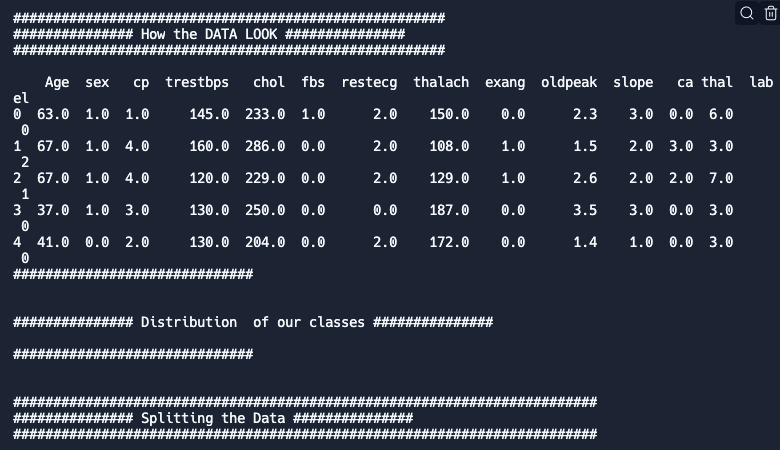 As you can observe, our data has an excel-like format: one line per data record (based on each patient) and columns that contain different types of information (e.g. age, sex, chest pain type…).
Q: Do you understand what each column represents?
- If not, how could you find out?
Task 5: Data Distribution
The distribution of our data can significantly affect the quality of our model. Thus, before we start training our model it’s important to understand how well-represented each class is in our dataset. The first simple way to do so is to create a histogram. For that, you need to run the following two lines. The first line calculates the histogram and the second one saves it as a pdf image under the folder “img”.
data.hist(column='label')
plt.savefig('img/hist.pdf')
Q: How does the distribution look like?
- What potential issues do you foresee?
Task 6: Splitting
Now it’s time to train our model. To train a machine learning model we need to split it into a training and a testing set (why?). An easy way to do that is to use the train_test_split function from sklearn.model_selection. This function receives as input the feature data and the label data and returns feature and label data for training and for testing. To split your data run the following line:
X_train, X_test, y_train, y_test = train_test_split(
  X, y, random_state=0, test_size=0.3) # 70% training and 30% test
The “test_size” determines what percentage of your data you will use for testing. To see how many records you use for training and testing after the split run the following code:
print("Training Features shape (X_train): " + str(X_train.shape))
print("Training Labels shape (y_train): " + str(y_train.shape))
print("Testing Features shape (X_test): " + str(X_test.shape))
print("Testing Labels shape (y_test): " + str(y_test.shape))
But how many records do we use per class in our training and testing datasets? To find out run the following lines:
print("\n ####  Save Histogram of Train/Test Label Counts ####")
y_train.hist()
y_test.hist()
plt.savefig('img/y_train_test_count.pdf')
print("Histogram Saved")
In the output, you can now see how many records are used per class. In addition, in your “img” folder you can check the y_train_test_count.pdf to see how the distribution of your labels looks like in the train and test datasets.
Feel free to change the test_size variable when splitting your data.
Q: Do you see a difference in your results? Do you understand the impact the way you split your data could have on your model performance?
Task 7: Training the Model
Now we can train our model. But which model should we train? Let’s start with two questions:
Q1: Should it be a classification or regression model?
Hint: Check what we are trying to estimate, a continuous value (e.g. temperature) or a class (e.g., “apple” vs “orange”).
Q2: Should we look at unsupervised or supervised models?
Hint: Is our dataset labeled or unlabeled?
Based on these questions we can scope down the potential models that we could use. Nowadays there is an abundance of available models and often researchers experiment with different ones. Here we will try 3 different models. To try these models you can use one of the following lines:
clf = DummyClassifier(strategy="constant", constant=0)

clf = KNeighborsClassifier(4)

clf = RandomForestClassifier(n_estimators=10)
Different models have different parameters that can be tuned. Feel free to experiment with the different models (or even other models of sklearn that are not mentioned here) and with using different parameters.
Q: How do we know which model and parameters work better for our problem?
- What are your expectations?
Task 8: Evaluation of the Model(s): Confusion Matrix
So let’s start evaluating our model. A good start is to calculate the confusion Matrix. Run the following lines to calculate the confusion matrix and store it as an image under the “img” folder:
plt.clf() # clear plot
fig = plt.figure(figsize=(6, 4))
ax = fig.add_subplot(111)
ConfusionMatrixDisplay.from_predictions(y_test, y_pred, cmap='Blues', ax=ax)
plt.savefig('img/confusion_matrix.pdf')
print("Saved the confusion matrix under the img folder\n")
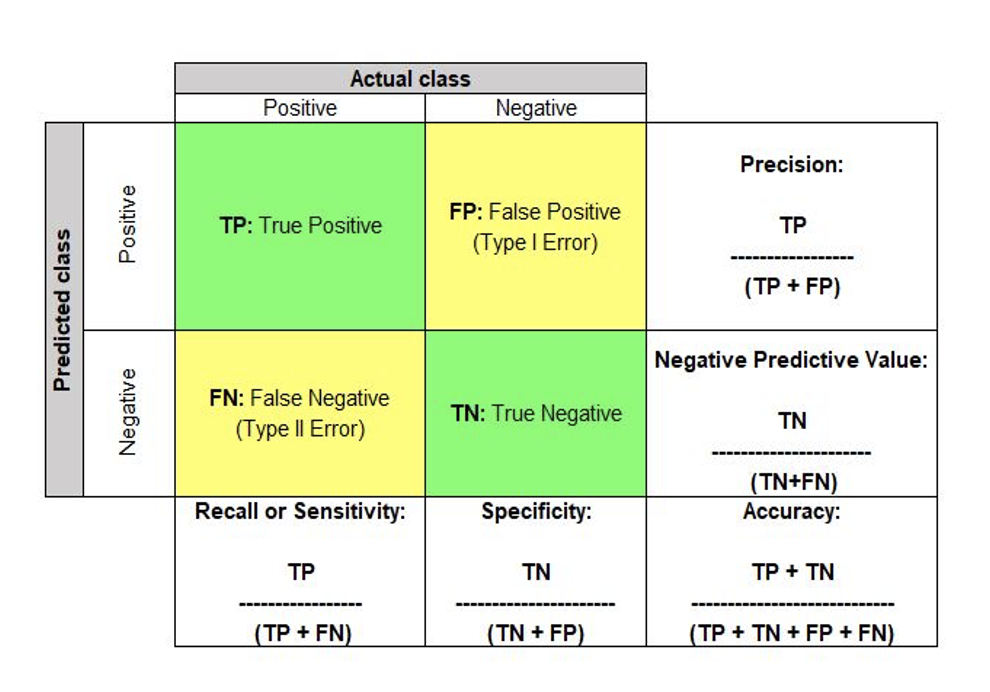
Q: Can you calculate the Precision and Recall of each class based on the confusion matrix?
- What’s more important when designing a system for predicting if a person has heart disease or not?
Fresh up your memory:
Task 9: Evaluation of the Model(s): Evaluation Metrics
What other metrics can we use to evaluate our model? As you already know, there are a variety of metrics that can be used. To select the one that fits your problem it is important to know how to “read” each metric. Sklearn has made it quite easy for us to calculate a group of the most often-used metrics. To do so run the following line:
print(classification_report(y_test, y_pred, target_names=labels))
If you now run your script you will see something like the following (numbers can differ):
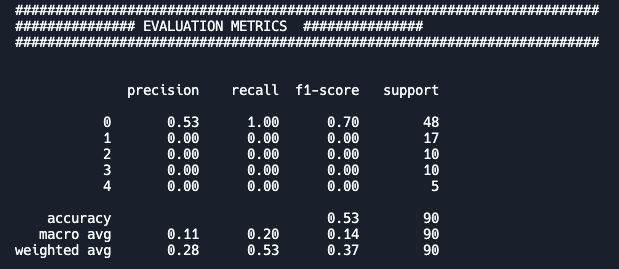
Q: What do the different columns and rows represent?
- Are the “macro” and “weighted” really needed? What do they show?
- Which evaluation metric fits our problem better?
Feel free to change the variables you have used above (e.g., how you split the data, what model you use, or the tuning parameters of each model) and reflect on how these changes affect your results.
Task 10: Evaluation of the Model(s): Cross-Validation
Do we exploit all our data? Wouldn’t it be better if we could train our model based on all the data?
Cross-validation allows us to train and test our model on the entire dataset. To perform cross-validation we do not need to split our dataset, but only separate the features from the labels. Run the following lines to perform cross-validation and print the evaluation metrics of your model.
scores = cross_validate(clf, X, y, cv=3, scoring=('accuracy', 'precision_micro', 'recall_macro',
 'f1_micro', 'f1_macro'), return_train_score=True)

printScores(scores)
Q: Why do we see three scores for each metric and not 4 (i.e., one for each of our classes)?
- Which evaluation metric fits our problem better?