Tutorial
In this section, our tutors will be on hand to assist you as you work through the assigned tasks. We’ll start the tutorial by revisiting the questions we posed in the “Preparation” section. Then, we’ll walk you through some examples using a new set of images to build a different application.
Recap
In the preparation, we emphasized the crucial significance of the background noise class in audio classification. This separate class recording helps improve the machine’s comprehension of the audio recording’s surroundings.
We have also raised a query regarding the requirement of background classes in image classification tasks. The answer to this question is clear - it is essential to include the background class for image classification. Without it, the background scene may be mistakenly identified as one of the classes defined, such as scissors or pens.
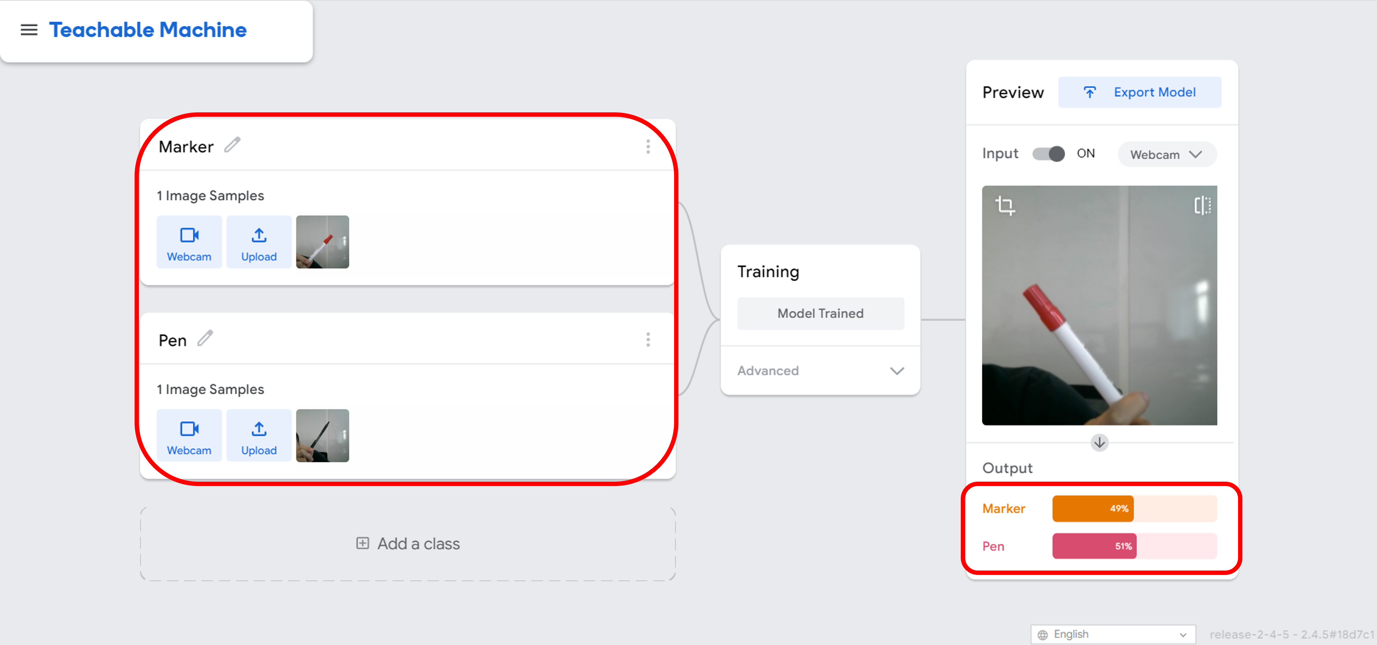
Let’s conduct an experiment using Teachable Machine. Our aim is to differentiate between a marker and a pen. As evidenced in the accompanying image, the machine performs exceptionally well even when the pen is not present in the original dataset.
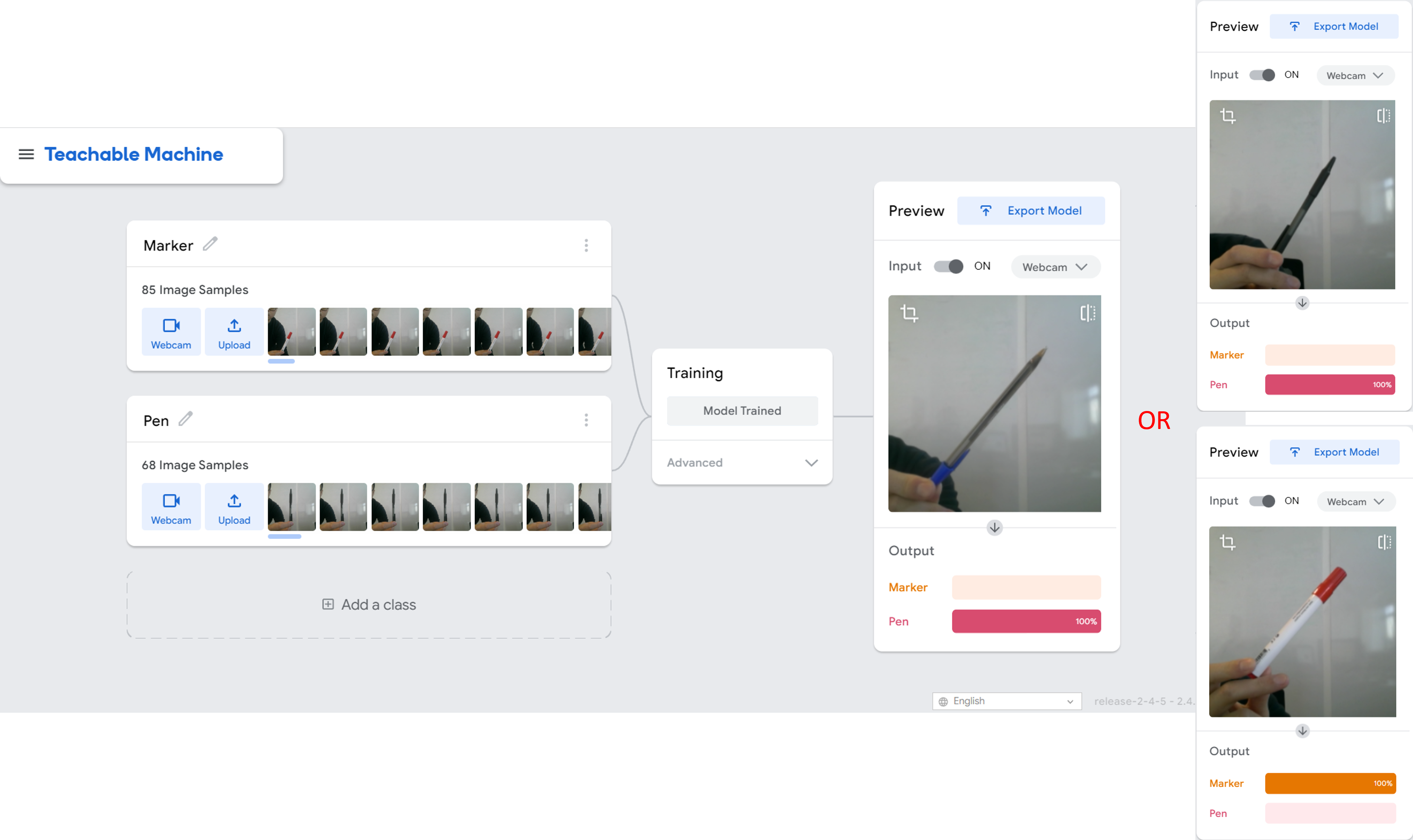
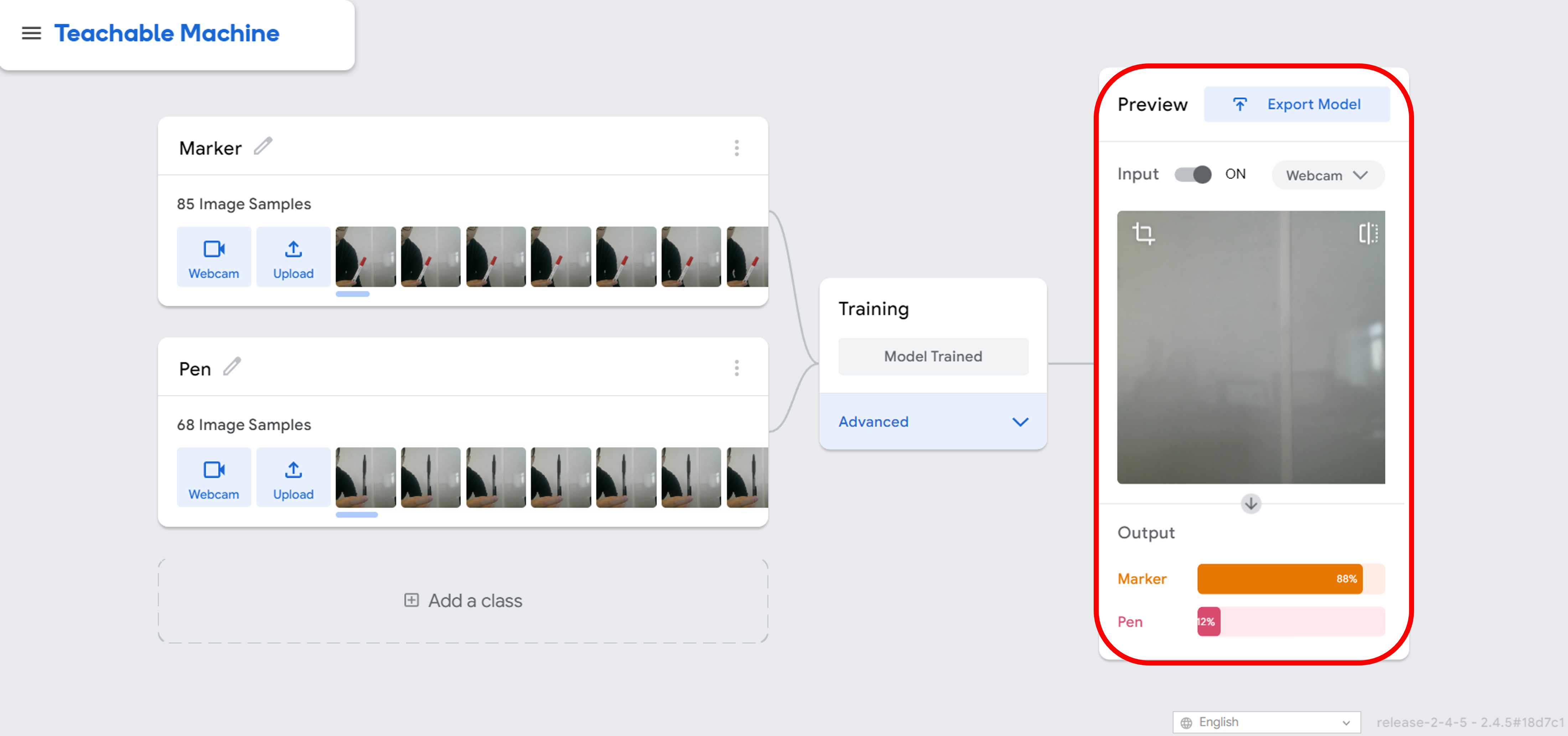
But, let’s consider the scenario where there is no pen or marker available. We can observe that the background has been forecasted as a marker with 80% confidence, but is that accurate?
This raises an issue for us, regarding how the model will perform if the dataset we supply is inadequate or flawed. How can we address misclassifications resulting from these imperfections?
Task 3: Imperfect Dataset
Here, we primarily focus on four issues that result in imperfect datasets: missing labels, inconsistent labels, incomplete dataset, and imbalanced dataset.
-
Missing labels: If some examples in the dataset do not have corresponding labels, the model may not be able to learn the correct relationships between the data and the labels, leading to reduced performance.
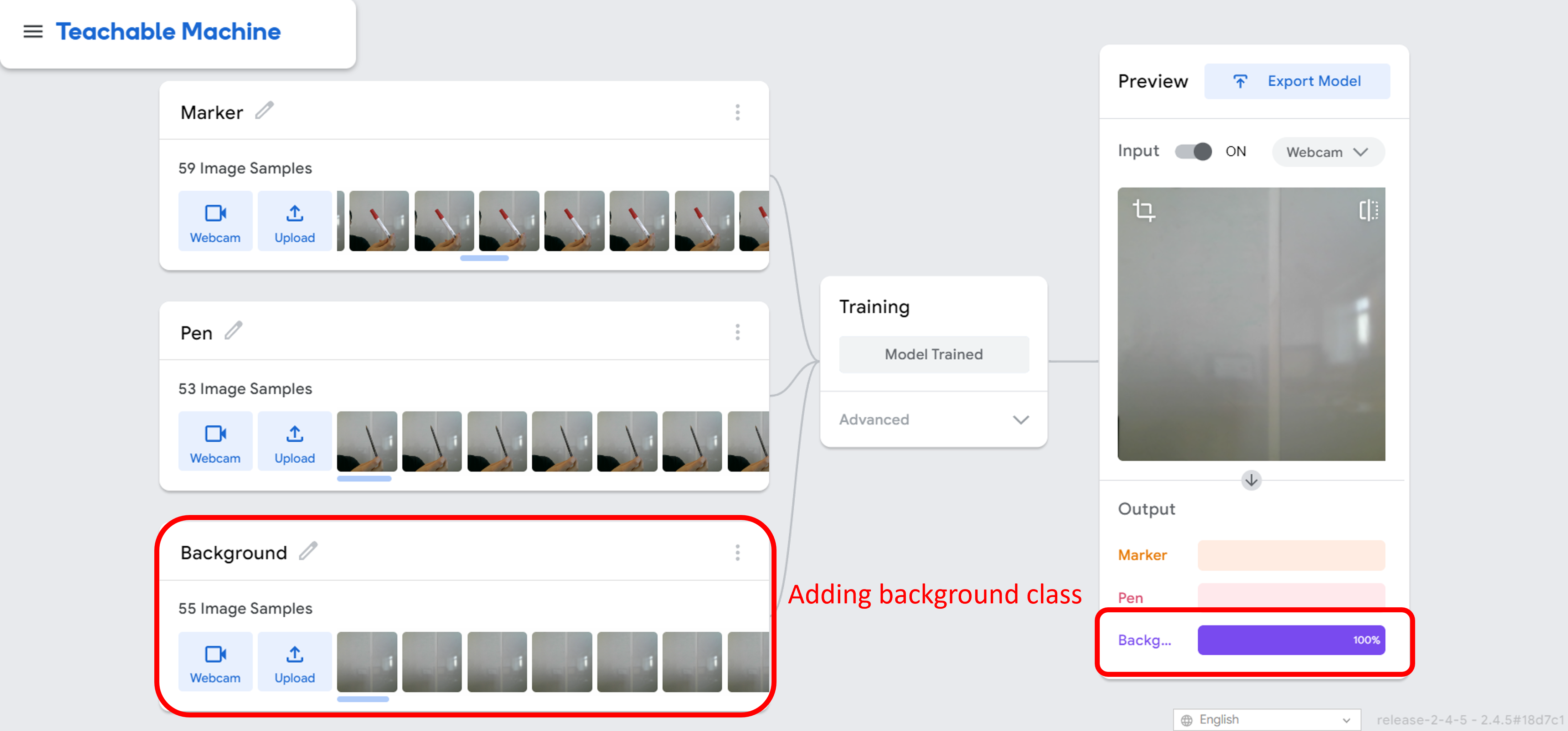
As outlined in the recap, the model we trained predicted the background scene as a marker if the background class was not defined. However, resolving this issue can be straightforward, by simply adding the missing classes to the original dataset.
-
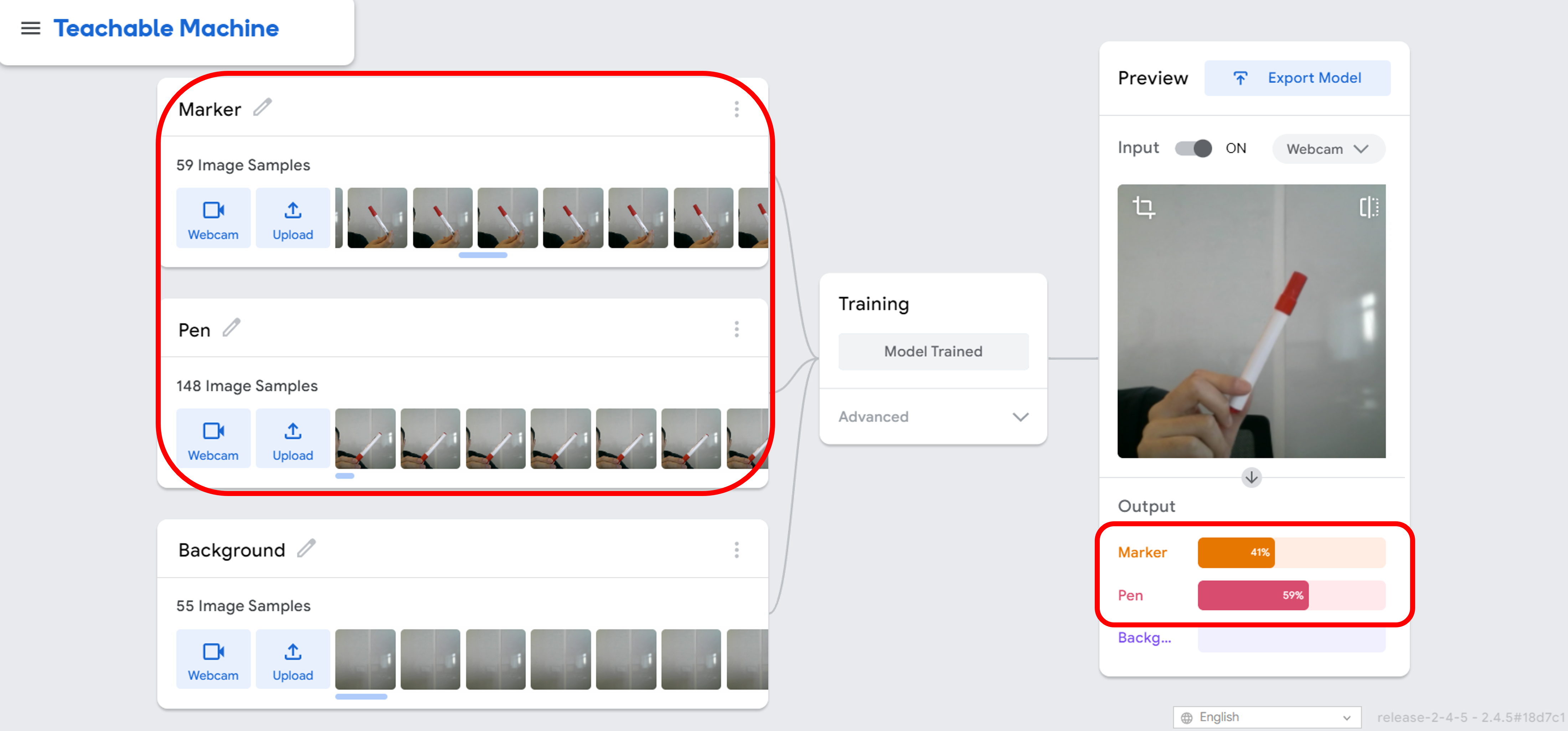
Inconsistent labels: If the labels in the dataset are inconsistent or incorrect, the model may learn incorrect relationships between the data and the labels, leading to inaccurate predictions.
Let’s examine the outcome if we include marker images within the pen class. The model will no longer be able to accurately predict whether the input image represents a pen or a marker.
How can we resolve the inaccuracies in predictions caused by inconsistent labels? A straightforward approach is data cleaning, where we remove or fix the inconsistent labels in the dataset to enhance the quality of the data.
-
Incomplete dataset: If the dataset does not contain enough examples or data points, the model may not be able to learn the patterns in the data, leading to underfitting or overfitting.
In this scenario, we have constructed a dataset consisting of only two images, one representing a marker and the other representing a pen. It becomes evident that the model struggles to predict the class to which the image belongs, owing to the limited training data. The lack of sufficient examples results in a model that lacks the ability to effectively learn the patterns and relationships between the data and the labels.
The solution to the problem of limited training data is quite straightforward. By including additional images in the dataset, the model will have a larger sample set from which to learn, allowing it to better comprehend the patterns and correlations between the data and the labels.
-
Imbalanced dataset: If the dataset is imbalanced, with more examples of one class than others, the model may learn to prioritize that class, leading to biased predictions.
We have constructed a database consisting of 34 images of markers and only 1 image of a pen. The result is clear, the model has a tendency to always predict that the input image is a marker. This is due to the fact that the model is heavily biased towards the marker class, as it has been exposed to 34 examples of markers compared to just 1 example of a pen.

This highlights the issue of imbalanced datasets and the need for a balanced distribution of classes in order to train a fair and accurate model. To resolve this issue, the solution is straightforward: simply add additional data to the classes that have insufficient samples. This will ensure that the model has a more diverse and representative training set, leading to better performance and more accurate predictions.
There are additional challenges that could arise in datasets, which you can be explored further after the tutorial, including:
- Outliers: If the dataset contains extreme values or outliers, the model may learn from these incorrect examples, leading to biased predictions.
- Non-representative data: If the dataset is not representative of the target population, the model may not be able to generalize to new data, leading to reduced performance.
Task 4 & 5 - Preparation
The aim of the following tasks is to distinguish between emergency vehicles and normal vehicles, utilizing a subset of AV Emergency Vehicle Classification Dataset. Please copy this notebook on Google Colab located here.
The code cells in the setup section of this Google Colab Notebook downloads a few folders folders, including:
- dataset: The folder contains data from the AV Emergency Vehicle Classification Dataset and has two subdirectories, one for the training data (train) and the other for the testing data (test).
- model: The folder holds the obtained Teachable Machine model (keras_model.h5), the corresponding class labels (labels.txt), and model project file (project.tm).
- The trained model could be accessed at https://teachablemachine.withgoogle.com/models/fVdKoKYt6/;
- Also, if you desire to re-create the model on the Teachable Machine website, you can upload the model project file (project.tm) to https://teachablemachine.withgoogle.com/train/.
- For information on how to export or download the Teachable Machine Model, please refer to the tutorial available at https://www.youtube.com/watch?v=n-zeeRLBgd0&ab_channel=ExperimentswithGoogle.
The “Function” section of the notebook is the core of Tasks 5 and 6, encompassing the introduction of noise to images and metrics to assess the performance of the Teachable Machine model.
Task 4: Noisy Image
We have discovered the consequences of constructing a dataset in an incorrect manner. However, what if the images themselves contain irrelevant or inconsistent information? This can also impact the performance of the model and lead to inaccurate predictions. The presence of noisy or irrelevant information can confuse the model, causing it to learn incorrect relationships between the data and the labels. Please follow the steps to modify the image according to the specified noise types.
-
Noise: Here, we simplify the image noise into a salt-and-pepper noise. Salt-and-pepper noise, also known as impulse noise, is a form of noise sometimes seen in digital images. This noise can be caused by sharp and sudden disturbances in the image signal. It presents itself as sparsely occurring white and black pixels, shown in the following image.
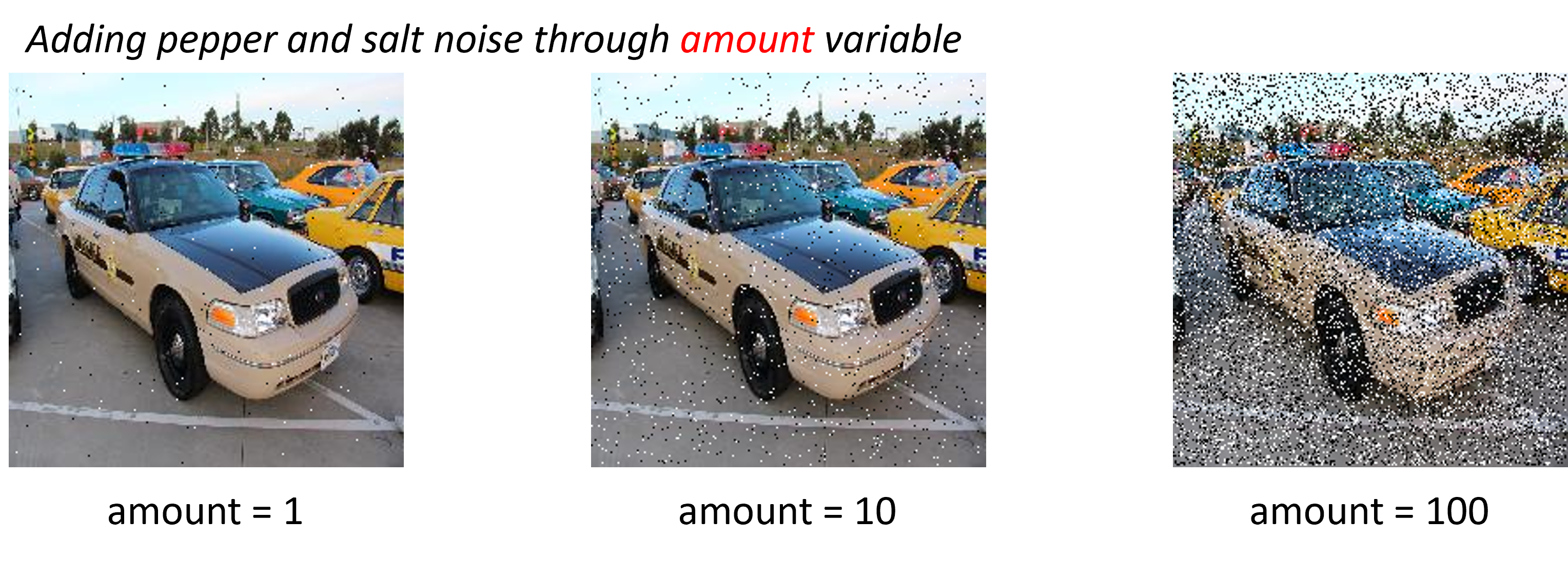
Navigate to the Noise section of the Colab notebook, and adjust the value of “amount” to observe how the image will change:
 # A function reads an image from the dataset/test/ folder.
 image = cv2.imread('/content/teachablemachine/dataset/test/1.jpg')

 # Adding salt and pepper noises to image.
 # By adjusting the value of the "amount" parameter, you can observe the effect on the image,
 # where higher values indicate a greater amount of noise added to the image.
 noise = adjust_noise(image, amount=10)
 # Plotting the image with added noise on the output tab
 plot(noise)
 # Save the image as 'saved_image.png' under Files tab by default.
 plot(noise, save_image=True)
After adding noise to the image, please upload it to Teachable Machine to observe how the prediction is affected.
-
Brightness: Brightness can also significantly impact the accuracy of image classification. If the images are too bright or too dark, it can lead to over-exposure or under-exposure, causing loss of important details in the image. This can result in the model being unable to accurately identify the features in the image, leading to misclassifications.
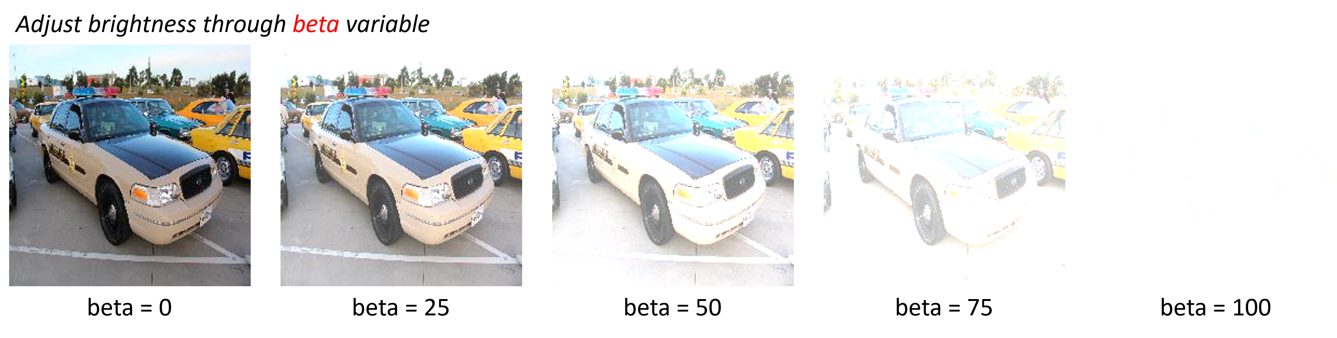
Navigate to the brightness section of the Colab notebook, and then adjust the value of “beta” to observe how the image will change:
 # # Adjusting the brightness of image.
 # # By adjusting the value of the "beta" parameter, you can observe the effect on the image,
 # # where higher values indicate a brighter image.
 bright = adjust_brightness(image, beta=50)
 # # Plotting the image with different brightness on the output tab
 plot(bright)
 plot(bright, True)
After adjusting the brightness of the image, please upload it to Teachable Machine to observe how the prediction is affected.
-
Partial Image: Partial images can significantly impact the accuracy of image classification. A partial image may contain only a portion of the object of interest and can be misleading to the classifier. The classifier may not have enough information to make an accurate prediction, resulting in a false positive or false negative.
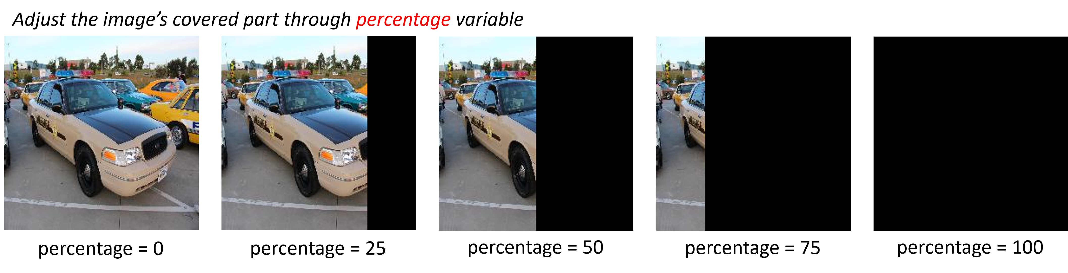
Navigate to the brightness section of the Colab notebook, and then adjust the value of “percentage” to observe how the image will change:
 # # Adjusting the covered areas of image.
 # # By adjusting the value of the "percentage" parameter, you can observe the effect on the image,
 # # where higher values indicate larger covered areas.
 partial = adjust_partial(image, percentage=60)
 # # Plotting the image with different covered areas on the output tab
 plot(partial)
 plot(partial, save_image=True)
After adjusting the partial covered areas of the image, please upload it to Teachable Machine to observe how the prediction is affected.
It is important to ensure that the data used in training the model is clean and relevant to the task at hand in order to achieve optimal performance.
Question: Could there be any other forms of noise that could impact the model’s predictions?
Task 5: Evaluation
Evaluation is the process of measuring the performance of a machine learning model. It involves comparing the predictions made by the model against actual, known outcomes to determine the accuracy of the model.
Why evaluation is important?
-
Measure model performance: Evaluation provides a way to measure the performance of the model and to compare it with other models. This allows us to determine which model is best suited for the task at hand.
-
Identify areas of improvement: Evaluation can help identify areas where the model needs improvement, such as high bias or high variance. This information can be used to make necessary adjustments to the model to improve its performance.
-
Evaluate model robustness: Evaluation helps to determine the robustness of the model and its ability to generalize well to new, unseen data. This is particularly important when deploying a model in real-world applications, where it must be able to handle a variety of inputs and situations.
What metrics we could use to evaluate model performance?
Question: Throughout Tasks 1 to 4, we manually uploaded images to assess the model’s accuracy. However, are there any metrics that can help us to evaluate the performance of a model in a systematic manner?
There are various evaluation metrics used in machine learning, that help to provide a comprehensive view of the model’s performance. If you would like to find more information about evaluation metrics: https://en.wikipedia.org/wiki/Confusion_matrix
The goal of this sub-task is to assess the performance of the Teachable Machine model that was trained in Task 4. To refresh our memory, the task scenario involves differentiating between emergency and normal vehicles.
Confusion Matrix: A confusion matrix is a table that is used to evaluate the performance of a machine learning model. It compares the predicted labels generated by the model with the actual, known labels to evaluate the accuracy of the model.
| Predicted condition | |||
|---|---|---|---|
| Total population = P + N |
Positive (PP) | Negative (PN) | |
| Actual condition | Positive (P) | True positive (TP) |
False negative (FN) |
| Negative (N) | False positive (FP) |
True negative (TN) | |
As we are attempting to distinguish emergency vehicles from normal vehicles, the positive predictions are considered to be the emergency vehicles. Therefore,
- True positive: the image depicts an emergency vehicle, and the classifier predicts it as an emergency vehicle;
- False negative: the image depicts an emergency vehicle, but the classifier predicts it as a normal vehicle;
- False positive: the image depicts a normal vehicle, but the classifier predicts it as an emergency vehicle;
- True negative: the image depicts a normal vehicle, and the classifier predicts it as a normal vehicle.
Here is a list of the actual results and the predictions made by the model for the 20 images located in the /dataset/test/ folder:
truth = ['Emergency vehicle', 'Emergency vehicle', 'Emergency vehicle', 'Emergency vehicle', 'Emergency vehicle', 'Emergency vehicle', 'Emergency vehicle', 'Emergency vehicle', 'Emergency vehicle', 'Emergency vehicle', 'Normal vehicle', 'Normal vehicle', 'Normal vehicle', 'Normal vehicle', 'Normal vehicle', 'Normal vehicle', 'Normal vehicle', 'Normal vehicle', 'Normal vehicle', 'Normal vehicle']
predicted = ['Normal vehicle', 'Emergency vehicle', 'Emergency vehicle', 'Emergency vehicle', 'Emergency vehicle', 'Emergency vehicle', 'Emergency vehicle', 'Emergency vehicle', 'Normal vehicle', 'Normal vehicle', 'Normal vehicle', 'Normal vehicle', 'Normal vehicle', 'Normal vehicle', 'Normal vehicle', 'Normal vehicle', 'Normal vehicle', 'Emergency vehicle', 'Emergency vehicle', 'Normal vehicle']
To create a visualization of the confusion matrix based on the results, navigate to the Evaluation section of the Colab notebook:
    # --- 5. Predict all images and prepare for confusion matrix ---
    folder_path = "/content/teachable-machine/dataset/test"  # Folder with images 1.jpg to 20.jpg
    y_true = []
    y_pred = []

    for i in range(1, 21):
        img_file = os.path.join(folder_path, f"{i}.jpg")

        # Determine true label
        if i <= 10:
            true_label = labels[0]  # First class
        else:
            true_label = labels[1]  # Second class

        predicted_label, confidence = predict_image(img_file)
        # print(f"{img_file} -> Predicted: {predicted_label}, Confidence: {confidence:.4f}")

        y_true.append(true_label)
        y_pred.append(predicted_label)

    # --- 6. Confusion matrix ---
    cm = confusion_matrix(y_true, y_pred, labels=labels)
    disp = ConfusionMatrixDisplay(confusion_matrix=cm, display_labels=labels)

    fig, ax = plt.subplots(figsize=(6,6))
    disp.plot(ax=ax, cmap=plt.cm.Blues, values_format='d')
    plt.title("Confusion Matrix")
    plt.show()
The visualized confusion matrix is shown in the following image.
